|
|
|
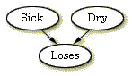
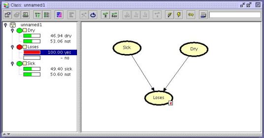
Figure 1: Bayesian network representing the Apple Tree problem. |
This tutorial shows you how to implement a small Bayesian network in the Hugin Graphical User Interface. The network we are about to implement is the one modeled in the Apple Tree example in the Bayesian Networks Tutorial.
The qualitative representation of our network is shown in
|
|
|
Figure 1: Bayesian network representing the Apple Tree problem. |
If you want to understand the design of this network, you should read about it in the Bayesian Networks Tutorial.
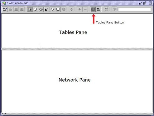
When you choose to start up the Hugin Graphical User Interface, the Main Hugin Window (or simply the Main Window) opens. This window contains a menu bar (called the Main Window Menu Bar), a tool bar (called the Main Window Tool Bar), and a document pane (called the Main Window Document Pane or simply the Document Pane). In the Document Pane, a new empty network called "unnamed1" is automatically opened in a network window (see Figure 2). It starts up in Edit Mode which allows you to start constructing the network immediately (the other main mode is Run Mode which allow you to use the network).
|
|
|
Figure 2: The network window containing a Tool Bar, a Tables Pane, and a Network Pane. |
The first thing we will do is add the Sick node. This can be done as follows:
When we have clicked in the Network Pane, a node labeled "C1" appears. We want to change this label to "Sick":
The "Name" is the internal name of the node while "Label" is the label of the node. If no label is specified (as was the case before we changed the label) the label used is the internal name. The internal name can consist of only the letters 'a'-'z' and 'A'-'Z', the digits '0'-'9', and the underscore character '_' while the label can be almost anything. Please note that the first character of the name must be a letter.
|
|
|
Figure 3: From left: The Discrete Chance Tool, the node properties tool, and the Link Tool. |
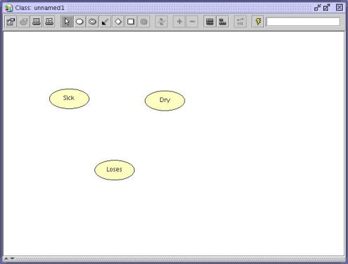
The Dry and Loses nodes are added the same way. We can add more nodes without having to press the Discrete Chance Tool all the time by holding down the SHIFT key while clicking in the Network Pane. When we have chosen a node in the Network Pane, we can access the node properties tool by holding down the right mouse button.
 |
|
Figure 4: The Network Pane contains the three nodes Sick, Dry, and Loses that have been added to the network. |
Now, we have a network similar to the one shown in the Network Pane
in
What we have now is the complete qualitative representation
which is similar to the one in
In the introduction to BNs the states of the nodes were specified as follows: Sick has two states: "sick" and "not", Dry has two states: "dry" and "not", and Loses has two states "yes" and "no".
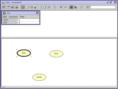
First, we open the Tables Pane by clicking the tables-pane button.
 |
|
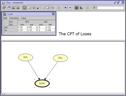
Figure 5: The CPT is opened by pressing the left mouse button over a node, while holding down the "ctrl" button. |
Next, we specify the states of Sick:
Now, do the same with Dry.
We can do exactly the same with Loses. Beware that the CPT of Loses is a little bigger than those of Sick and Dry. This is just because Loses has parent nodes (Sick and Dry don't).
The next step is to enter the CPT values correctly (as default, the Hugin Graphical
User Interface
has given all nodes a uniform distribution). The values were specified in the introduction to BNs and they are shown in
|
||||
| Table 1: P(Sick). |
|
||||
| Table 2: P(Dry). |
|
|||||||||||||||||||
|
Table 3: P(Loses | Sick, Dry). |
|||||||||||||||||||
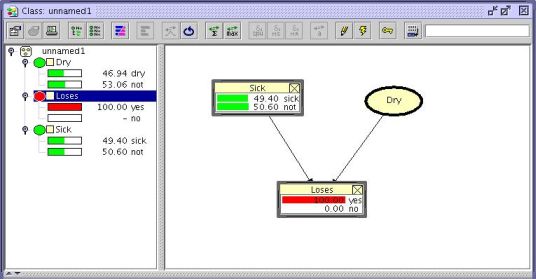
First, we select all three nodes (shortcut: Ctrl+A) to get the CPTs displayed in the Tables Pane. Next, we enter the values into the Sick node:
Enter the values for Dry and Loses the same way. When you have entered the
CPT for Loses, the network window should look like
|
|
| Figure 6: The network window with node Loses selected. The CPT of Loses appears in the Tables Pane. |
This completes the construction of the network. At this point it would be a good idea to save the network. Here is how to do it:
Now, let's compile the network and see how it works:
| Figure 7: The Run Mode tool button. |
The compiler checks for the following errors:
If you have done exactly as this tutorial told you, there should not be any errors in the compilation process. The compilation should be finished very fast with a small network like ours. After the compilation, the Run Mode is entered (we have so far only been working in Edit Mode).
Running in Run Mode, the network window is split into two by
a vertical bar (see
|
|
| Figure 8: The network window in Run Mode. To the left is the Node List Pane (having Loses and Sick expanded) and to the right is the Network Pane. |
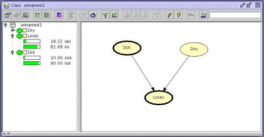
We can view the probabilities of a node being in a certain state by expanding the node in the Node List Pane. We expand (collapse) a node by clicking its expand (collapse) icon in the Node List Pane, by double-clicking its node symbol in the Node List Pane, or by selecting (deselecting) it in the Network Pane. We can also expand (collapse) all nodes at once by pressing the expand (collapse) node list tool in the Tool Bar just to the right of the node properties tool.
Now, imagine that we want to use our network to find the probability of an apple tree being sick given the information that the tree is losing its leaves. This is done as follows:
| Figure 9: The Sum Propagation Tool. |
This should give the output shown in
|
|
| Figure 10: Our network after the evidence that the tree is losing its leaves has been entered and propagated. |
The probability of the tree being sick is now 0.49.
If you do not read the value specified above, you have probably mistyped something when filling in the CPTs. Then please check the CPTs of all the nodes.
In the last section, we used the Node List Pane to enter evidence and retrieve beliefs. We can also do this by using the monitor windows. The monitor windows show the same information as the Node List Pane but we have the opportunity to place the monitor windows near the corresponding nodes of the network in the Network Pane. We can open a monitor window for each node in the Network Pane, but the best way to use them is probably only to open a monitor window for the nodes in the network which have special interest. Otherwise, they might take up too much space.
Now, we shall open monitor windows for Sick and Loses and repeat the computations from before. First, initialize the network:
Then, we are ready to open the monitor windows of Sick and loses.
|
|
|
Figure 11: Monitor windows of Sick and loses shown in the Network Pane. |
The rest of this tutorial introduces some very useful aspects of the Hugin Graphical User Interface, but it can be skipped.
From the propagation in the previous section we could see that the probability of the apple tree suffering from drought is 0.47. In both the case of Sick and Dry it is more likely that the state is "not". This could make one believe that the most likely combination of states is when both Sick and Dry are in state "not". However, this is a wrong conclusion. If we want to find the most likely combination of states in all nodes, we should use max propagation (in stead of sum propagation). The Max Propagation Tool is found in the Tool Bar just to the right of the Sum Propagation Tool.
Now, try to press the Max Propagation Tool. In each node, a state having the value 100.00 belongs to a most likely combination of states. In this case, this gives one unique combination being the most likely: Sick is "sick" and Dry is "not"
We see that even if Sick="sick" is less likely than Sick="not", Sick="sick" is contained in the most likely combination of the states of the nodes while Sick="not" is not. This shows that we need to be careful in making conclusions from the result of a propagation.
Now, one might want to know the probability of this most likely combination of states (or of any other combination of states) under the assumption that the entered evidence holds.
Here, we shall describe a technique to compute the probability of the most likely combination of states given the evidence that the apple tree is losing its leaves. This probability is written:
Each time we perform sum propagation in a network, the probability of the entered evidence is shown in the lower left corner of the Hugin Graphical User Interface window (the value). If we have chosen the "yes" state of the Loses node and performed sum propagation, we can read the probability of Loses="yes" (written ). This value should be 0.1832.
The technique uses the following rule from probability theory (known as the fundamental rule):
The only kind of probability we can get from Hugin is the probability of a series of pieces of evidence which can be written in the form:
We use the fundamental rule to rewrite our requested probability to some expression composed by such components:
In the fundamental rule, we have divided both sides with . Then we have substituted A with and B with .
We already know so we only need to
compute
This value should be 0.081. Now, we are ready to compute the requested probability:
So, the probability of the most likely combination of states of Sick and Dry, given that Loses="yes", is 0.442.