 |
| Figure 1: The BN constructed in the Introduction to BNs. |
A (limited memory) influence diagram (ID) may be used instead of a Bayesian network (BN) if you wish to explicitly model various decision alternatives and the utilities associated with these. To some extent it is possible to construct a model for decision making with a pure BN, but the concepts of utility and decisions are not explicitly covered. An influence diagram is simply a BN, extended with utility nodes and decision nodes. Having these two new types of nodes, we also need to have a name for the old node type. We shall call these nodes chance nodes.
We shall present the concept of influence diagrams by extending the BN constructed in the apple tree example from the Introduction to BNs.
Again, we consider the Apple Tree Example (see Figure 1).
 |
| Figure 1: The BN constructed in the Introduction to BNs. |
Apple Jack now wants to decide whether or not to invest resources in giving the tree some treatment. Since this involves a decision through time, we have to modify the BN into a dynamic one as described in the Introduction to BNs section. We first add three nodes very similar to those already in the network. The new nodes Sick', Dry', and Loses' represent the same as the old nodes - except that they represent the situation at the time of harvest. These nodes have been added in Figure 2.
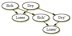 |
| Figure 2: Addition of similar nodes representing the harvest time expectations of the state of the tree. |
The new nodes can be in the same states as the old nodes: Sick' can be either "sick" or "not" - Dry' can be either "dry" or "not" - and Loses' can be either "yes" or "no". In the new model, we expect a causal dependence from both the old Sick node to the new Sick' node and the old Dry node to the new Dry' node. This is because if, for example, we expect the tree to be sick now, then this is also very likely to be the case in the future. Of course the strength of the dependence depends on how far out in the future we look. Perhaps one could also have a dependence from Loses to Loses' but we have not done so in this model.
Apple Jack has the opportunity to do something about his problem. He can try to heal the tree with a treatment to get rid of the possible sickness. If he expects that the losing of leaves is caused by drought, he might save his money and just wait for rain. The action of giving the tree a treatment is now added as a decision node to the BN which will then no longer be a BN. Instead it will be the influence diagram shown in Figure 3. Action nodes are represented by rectangles.
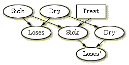 |
| Figure 3: Addition of a decision node for treatment. |
The Treat decision node has the states "treat" and "not". As it appears from Figure 3, we have added a link from Treat to Sick'. This is because we expect the treatment to have an impact on the future health of the tree.
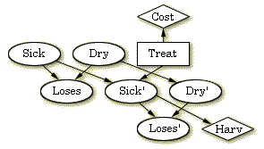
Before the influence diagram is completed, we need to specify the utility function enabling us to compute the expected utility of a decision. This is done by adding utility nodes to the diagram, each contributing with one part of the total utility. The utility nodes are added in Figure 4. Utility nodes are represented by diamonds.
 |
|
Figure 4: The complete qualitative representation of the (limited memory) influence diagram used for decision making in Apple Jack's orchard. |
The utility node Cost gathers information about the cost of the treatment while Harv represents the utility at the time of the harvest. It depends on the state of Sick' indicating that the production of apples depends on the health of the tree.
Figure 4 shows the complete qualitative representation of the influence diagram. To get the quantitative representation as well, we need to construct a conditional probability table (CPT) for each chance node and a utility table for each utility node. A decision node does not have any table.
The following tables show one way of how the CPTs of the chance nodes could be specified.
|
||||
| Table 1: P(Sick). |
|
||||
| Table 2: P(Dry). |
|
|||||||||||||||||||
| Table 3: P(Loses | Sick, Dry). | |||||||||||||||||||
|
|||||||||||||||||||
| Table 4: P(Sick' | Sick, Treat). | |||||||||||||||||||
|
|||||||||
| Table 5: P(Dry' | Dry). |
|
|||||||||||||||||||
| Table 6: P(Loses' | Sick', Dry'). | |||||||||||||||||||
The following tables show how the tables of the utility nodes could be specified in USD.
|
||||
| Table 7: U(Harv). |
|
||||
| Table 8: U(Cost). |
The utility tables are simply cost functions. Table 7 can be interpreted as if we have healthy tree (Sick' is in state "not"), then Apple Jack will get a $20000 income, while if the tree is sick (Sick' is in state "yes") Apple Jack's income will be only $3000. Table 8 shows that to treat the tree, Apple Jack has to spend $8000. The purpose of our influence diagram is to be able to compute the action of the Treat node giving the highest expected utility. This is a very tricky job if you are to do it without the help from a computer and we shall not do it here. In stead, we suggest that you now try to go through the two tutorials describing how to implement this influence diagram in the HUGIN Graphical User Interface and let it do the computations. Also, you might be interested in learning more about the semantics of (limited memory) influence diagrams.
An (limited memory) influence diagram is a Bayesian network augmented with decision and utility nodes (the random variables of a limited memory influence diagram are often called chance variables). The limited memory influence diagram relaxes two fundamental assumptions of the traditional influence diagram: the non-forgetting assumption and the total order on decisions.
We are interested in making the best possible decisions for our application. We therefore associate utilities with the state configurations of the network. These utilities are represented by utility nodes. Each utility node has a utility function that to each configuration of states of its parents associates a utility. (Utility nodes do not have children). By making decisions, we influence the probabilities of the configurations of the network. We can therefore compute the expected utility of each decision alternative (the global utility function is the sum of all the local utility functions). We shall choose the alternative with the highest expected utility; this is known as the maximum expected utility principle.
Relaxing the non-forgetting assumption and the total order on decisions implies a significant change in the semantics of a LIMID compared to a traditional influence diagram. In a LIMID it is necessary to specify for each decision the information available to the decision maker at that decision. There are no implicit informational links in a LIMID.A link into a decision node specify that the value of the parent node is known at the decision.
The computational method underlying the implementation of limited memory influence diagrams in the HUGIN Decision Engine is described by Lauritzen & Nilsson (2001). The algorithm used is known as Single Policy Updating.
As another example, consider the following decision scenario:
|
An oil wildcatter must decide whether or not to drill. He is uncertain whether the hole is dry, wet, or soaking. At a cost of $10,000, the oil wildcatter could take seismic soundings which will help determine the underlying geological structure at the site. The soundings will disclose whether the terrain below has closed structure (good), open structure (so-so), or no structure (bad). |
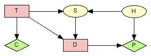
This decision scenario can be represented by the influence diagram of Figure 5, where T represents the decision on whether or not to test; D represents the decision on whether to drill or not to drill; S represents the outcome of the seismic soundings test (if the oil wildcatter decides to test); H represents the state of the hole; C represents the cost associated with the seismic soundings test; and P represents the expected payoff associated with drilling.
 |
|
Figure 5: An influence diagram for the oil wildcatters decision problem. |
The cost of drilling is $70,000. If the oil wildcatter decides to drill, the expected payoff (i.e., the value of the oil found minus the cost of drilling) is $-70,000 if the hole is dry, $50,000 if the hole is wet, and $200,000 if the hole is soaking; if the oil wildcatter decides not to drill, the payoff is (of course) $0.
The experts have estimated the following probability distribution for the state of the hole: P(dry)=0.5, P(wet)=0.3, and P(soaking)=0.2. Moreover, the seismic soundings test is not perfect; the conditional probabilities for the outcomes of the test given the state of the hole are:
|
On the basis of this (limited memory) influence diagram, the HUGIN Decision Engine computes the utility associated with testing to be $22,500 and the utility associated with not testing to be $20,000. The optimal strategy is to perform the seismic soundings test, and then decide whether to drill or not to drill based on the outcome of the test.
Notice that the informational link from node T to node D is of outmost importanct. The LIMID relaxes the non-forgetting assumption of the traditional influence diagram. This implies that for each decision node it is necessary (and very important) to specify exactly the information available to the decision maker. No informational links can be assumed implicitly present in the network.
[This example is due to Raiffa (1968). A more thorough description of this example is found in the Examples section.]
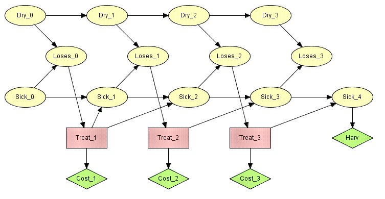
The LIMID in Figure 4 representing the decision problem of Apple Jack assumes a single decision with no observations made prior to the decision. In a more realistic setting Apple Jack is likely to monitor the tree over a period of time such as each day. Assume he prior to making a decision on treating the tree observes whether or not the tree is loosing its leaves. Each day he observes if the tree is loosing its leaves and makes a decision on the treatment irrespectively of what he did the previous day. We may use a limited memory influence diagram to model this situation.
 |
|
Figure 6: A limited memory influence diagram for Apple Jack with multiple decisions. |
Figure 6 shows a limited memory influence diagram for the situation described above where Apple Jack monitors the tree for three days before harvest. The informational links of the diagram specifies that Apple Jack each day observes whether the tree is (still) loosing its leaves, but otherwise neither recalls the observations nor the decisions made at previous time steps.
The solution to the LIMID is a strategy consisting of one policy for each decision. The policy is a function from the known variables to the states of the decision. It is not a function of all past observations as the decision maker is assumed only to know the most recent observation on loses leaves. This is different from the traditional influence diagram where the policy would be a function from all past observations and decisions as the decision maker is assumed to be non-forgetting.
In the example there is a total order on the decisions. This need not be the case in general.
To learn how to build a LIMID using the Hugin Graphical User Interface, please consult the How to Build LIMIDs tutorial. Also, you might be interested in learning more about the semantics of (limited memory) influence diagrams and the associated constraints imposed on their usage.