|
|
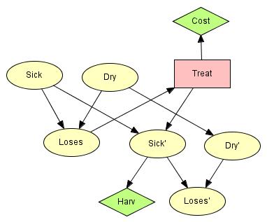
| Figure 1: The qualitative representation of the influence diagram used for decision making in Apple Jacks plantation. |
This tutorial shows you how to implement a small influence diagram in the Hugin
Graphical User Interface. It requires that you have already constructed the Bayesian network
from the How to Build a Bayesian Network Tutorial. The influence diagram you are
about to implement is the one modeled in the Influence Diagrams
Tutorial. It
helps plantation owner Apple Jack to decide whether or not to give his apple tree, which
is losing its leaves, some treatment. The qualitative representation of the
influence diagram is shown in
|
|
| Figure 1: The qualitative representation of the influence diagram used for decision making in Apple Jacks plantation. |
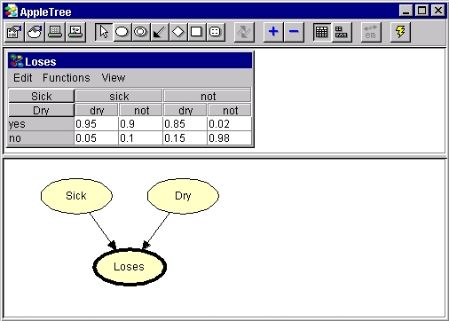
First, you must open the network constructed in the How to Build BNs tutorial if it is not already open. Here is how to do it:
In
|
|
|
Figure 2: The Network Window in Edit Mode with the network from the How to Build BNs tutorial. |
In the influence diagram in
The Hugin Graphical User Interface generates new names and labels for the new nodes. You can keep the names and change the labels to Sick', Dry', and Loses' (you cannot use "Sick'" as the name because it contains the prime character which is illegal in names):
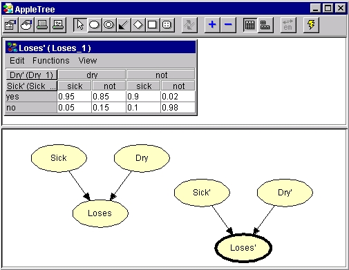
Perform the steps above for all three new nodes. Your network should
then look as the one in
|
|
|
Figure 3: The network extended with Sick', Dry', and Loses'. |
The next step is to add causal links from Sick to Sick' and from Dry to Dry':
Holding down the SHIFT key enables you to create more causal links sequentially without having to reactivate the Link Tool.
So far, the network we have constructed is still a Bayesian network. Now, we shall
make the first change that makes it an influence diagram. This change is the addition of a
utility node. The utility node we shall add is the Harv node (see
The harvest depends on the state of Sick' and thus there is an link from Sick' to Harv. Add this link:
The utility of the harvest was specified to that found in
|
||||
| Table 1: U(Harv). |
You enter the values of
Now, you are about to add the decision node Treat (see
You add an action to a decision node in the same way as you add a state to a chance node:
The Treat decision node has an impact on the Sick' node so:
The new decision node represents the decision to give the tree some
treatment or not. If the plantation owner (Apple Jack) chooses to give treatment this will
cost him something which shall be modeled by the Cost utility node. The Cost
node has the utility table shown in
|
||||
| Table 2: U(Cost). |
Now, add the Cost utility node to the influence diagram:
When we copied the nodes Sick' and Dry', they inherited
the CPTs of Sick and Dry. However, as both these nodes have become children
of other nodes, their CPTs are no longer correct. Their new CPTs were specified to those
found in
|
|||||||||||||||||||
|
Table 3: P(Sick' | Sick, Treat). |
|||||||||||||||||||
|
|||||||||
|
Table 4: P(Dry' | Dry). |
Now, your (limited memory) influence diagram (LIMID) is finished and it should look like the one
in
|
|
| Figure 4: The complete influence diagram. |
You can now try out the LIMID. First, compile the LIMID:
The compilation of an influence diagram may produce some of the same errors as described in the How to Build BNs tutorial. If the LIMID does not compile, you have probably made some minor error. Once the influence diagram has been compiled, probabilities and expected utilities are computed under the initial policy. To solve the influence diagram it is necessary to invoke Single Policy Updating.
When the LIMID has been compiled, you should do a Single Policy Updating. Now, imagine that the only thing Jack knows about his tree is that it is losing leaves. Then, what will be the best thing for him to do? To find out this, follow these steps:
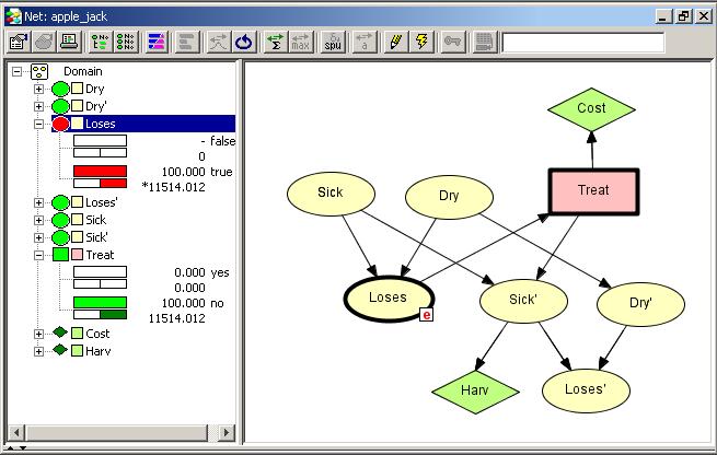
You should be reading something looking like that in
|
|
| Figure 5: The influence diagram propagated with the evidence that Loses="yes". |
You read 11514 as the expected utility of doing nothing. This suggests that it will be best for Apple Jack not to treat the tree.
This finishes the tutorial. You should now be able use the Hugin Graphical User Interface to construct your own (limited-memory) influence diagrams. However, if you want to create large and complex models, you should study the area more than just reading this tutorial.
Please read the document semantics of LIMID to learn more about LIMIDs.