 |
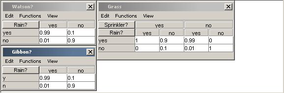
| Figure 1: Tables displayed in framed mode |
The Hugin Graphical User Interface provides a number of powerful features for displaying node tables, including resizing, collapsing selected sets of columns, graphics display modes, etc. Furthermore, the user can choose between two different ways of organizing the tables:
|
| Figure 1: Tables displayed in framed mode |
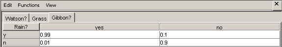 |
| Figure 2: Tables displayed in tabbed mode |
The framed mode has the advantage that several tables can be viewed at once, whereas the tabbed mode is a lot more compact (with several open tables) and it is easier to navigate the tables. The preferred table mode can be set in the Preferences, and it can be changed by selecting the "Toggle Table Mode" item in the View Menu of a table.
The probabilities and utilities of discrete chance nodes and utility nodes, respectively, can be specified manually (i.e., directly through click-and-type operations) or they can be specified indirectly through specification of powerful expressions, which (if appropriate) can save a lot of work. The initial policy for a decision node can also be specified both manually and using expressions.
For all four kinds of tables, there is a menu bar containing an Edit menu, a Functions menu, and a View menu.
When working in Edit Mode with the Tables Pane open, the currently selected nodes will have their tables displayed in the Tables Pane.
For discrete chance nodes, discrete decision nodes, and utility nodes the node table has two different modes:
 |
|
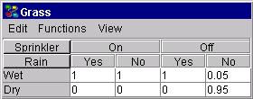
Figure 1: A CPT in manual mode. |
 |
|
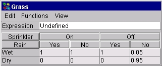
Figure 2: A CPT in expressions mode. |
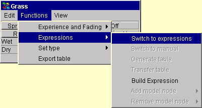
To switch between the two modes, select the appropriate item in the Functions menu of the node table, see Figure 3.
 |
|
Figure 3: Selection of Expressions mode. |
In Expressions mode there are one or more editable text fields in which expressions can be specified (one in each text field) either manually or through the Expression Builder. The number of text fields available depends on the number of states of the model nodes. If no model nodes have been specified, there will only be one text field (i.e., the same expression is used for all parent configurations).
For discrete chance node this function expresses a conditional probability distribution over the states of the node for each configuration of the states of the parents of the node, which are also discrete chance nodes. The conditional probability distribution (or marginal probability distribution in case of no parents) is represented as a conditional probability table (abbreviated CPT). Figure 4 shows an example of a CPT for the node Grass with parents Rain and Sprinkler.
|
|
|
Figure 4: The CPT of node Grass with parents Rain and Sprinkler. |
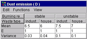
For each continuous chance node with discrete parents I and continuous parents Z, the function expresses a (one-dimensional) Gaussian distribution conditional on the values of the parents:
![]()
[This is known as a CG distribution.] Note that the mean depends linearly on the continuous parents and that the variance does not depend on the continuous parents. However, both the linear function and the variance are allowed to depend on the discrete parents. (These restrictions ensure that exact inference is possible.) Thus, for each configuration of the discrete parents, a mean and a variance parameter must be specified, as well as a regression parameter for each continuous parent. Figure 5 shows the table for the continuous node Dust Emission (Emission) with discrete parents Burning Regimen (Burn) and Waste (Waste Type), and the continuous parent Filter Efficiency (Efficiency).
|
|
|
Figure 5: The table for continuous node Emission with parents Burn and Waste. |
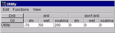
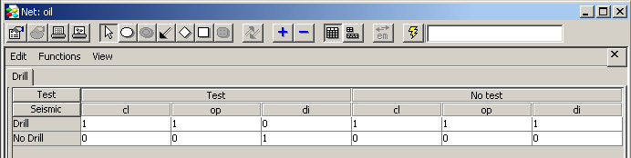
For each utility node, the function associated with the node expresses a utility function, where a utility value has to be specified for each configuration of its parents, which can be discrete chance and decision nodes. Figure 6 shows the table for the utility node Utility with the discrete chance node Oil and the discrete decision node Drill as parents.
|
|
|
Figure 6: The table for utility node Utility with parents Drill and Oil. |
For each decision node is associated a decision table, which is an encoding of the initial policy for the decision node. Figure 7 shows the table of a decision node, D, with decision options "Drill" and "No Drill".
 |
| Figure 7: The decision table of a decision node D. |
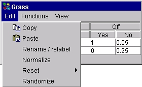
The Edit menu provides the following functionalities (see Figure 8):
Please note that the copy and paste operations also work across applications (e.g., to/from the Hugin node table from/to Excel, Word, Emacs, etc.).
|
|
|
Figure 8: Edit menu for the node table. |
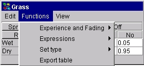
The Functions menu provides the following functionalities (see Figure 9):
|
|
|
Figure 9: Functions menu for the node table. |
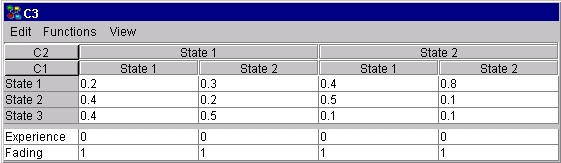
|
|
|
Figure 10: Experience and fading tables created and shown. |
The View menu provides the following functionalities (see Figure 11):
|
|
|
Figure 11: View menu for the node table. |
- Normal mode in which only the numbers are displayed.
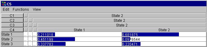
- Bar mode in which each number is overlaid by a bar of length corresponding to the number (see Figure 16).
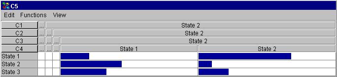
- Pure bars mode in which only the bars are shown (see Figure 17).
- Auto normalize can be turned on, meaning that when dragging a bar the other bars belonging to the distribution are automatically adjusted to make sure the numbers (represented by the bar lengths) sum to 1.
See the next section for more details on display modes.
When the Tables Pane is open, the tables for the nodes selected in the Network Pane will be displayed. The Hugin Graphical User Interface has a number of powerful features for displaying node tables:
A node table frame (i.e., the internal window displaying the table) can be resized arbitrarily by clicking and holding (i.e., dragging) the left mouse at the border of the frame. The width of the cells of the table resizes correspondingly. The width of the first column (containing parent and state names) can be resized by dragging the left mouse button at the border between the first and the second column. This can be useful if the parent and/or state names are very long or very short.
The order of appearance of the parents in the node table can be changed in Table tab of the Node Properties pane. This can be useful for grouping together sets of distributions.
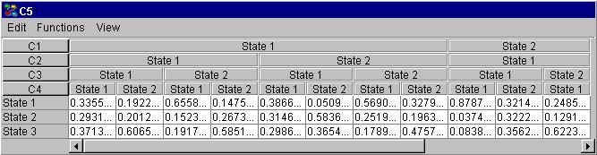
Also, for better viewing of selected sets of distributions, sets of columns (corresponding to sets of parent configurations) can be collapsed by double-clicking the appropriate labels for parent states. Figure 12 shows (part of) the table for node C5 with parents C1, C2, C3, and C4. Now, suppose we're interested in working with the probability distributions for C1 in state "State 2". One option would be to use the horizontal scroll bar. Another, much easier and more convenient approach would be to collapse the part of the table where C1 is in state "State 1". This can be achieved by double-clicking the text field labeled "State 1" in the C1 row.
|
|
|
Figure 12: The table for node C5 with all columns collapsed for which the state of parent node C1 equals "State 2". |
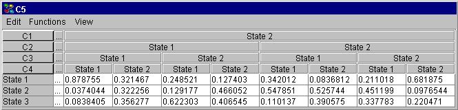
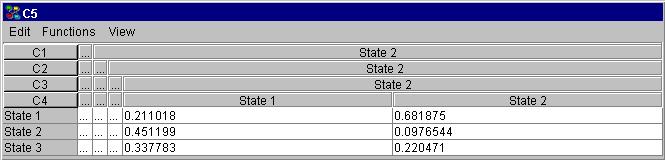
Figure 13 shows the resulting table. Note that the width of the cells has changed, allowing us to see all digits after the decimal point. Likewise, we can collapse other columns. In general, the cells in the parent states section can be double-clicked for all parent rows but the last, making the corresponding columns collapse. Figure 14 shows the table with all columns collapsed where the states for all parent nodes but C4 equals "State 1".
|
|
|
Figure 13: The table for node C5 with all columns collapsed for which the state of parent node C1 equals "State 1". |
|
|
|
Figure 14: The table for node C5 with all columns collapsed for which the states of parent nodes C1, C2, and C3 equal "State 1". |
A collapsed column can be expanded by double-clicking the top cell of the column.
Please note that when changing the order of appearance of the parents (see above), any collapsed columns will be expanded.
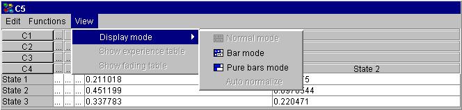
Sometimes, viewing or even specifying probability distributions graphically instead of numerically is preferable. The Hugin Graphical User Interface allows the user to select among three different display modes: The numerical mode (denoted the Normal mode), the numerical and graphics mode (denoted the Bar mode), and the graphics mode (denoted the Pure bars mode). The desired mode can be selected under the View menu, see Figure 15.
|
|
|
Figure 15: The probabilities of a table for a discrete chance node can be displayed numerically, graphically, or both numerically and graphically. |
Figures 16 and 17 show the table of Figure 14 in Bar mode and Pure bars mode, respectively.
|
|
|
Figure 16: The CPT for node C5 displayed in Bar mode. |
|
|
|
Figure 17: The CPT for node C5 displayed in Pure Bars mode. |
Graphical specification of probabilities is performed by dragging the bars with the left mouse button. When Bar mode or Pure bars mode have been selected, the distributions can be set to auto-normalize when the probabilities are changed. This feature can be selected under the Display mode submenu of the View menu.
Please note that the graphical viewing and specification mode is available only in tables for discrete chance and decision nodes.